With added pressure in realizing the semester is half over, as well as an upcoming interview for a position dealing with DSP and machine learning, I came into this week with newfound motivation. The focus that comes with a little bit of pressure is paradoxically quite freeing.
I had some issues when attempting to compare features between audio files. In hindsight, it was an obvious mistake that I had already learned in theory. But of course, applying theoretical knowledge always reveals the points of weak understanding.
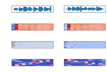
As I’ve written in the past, MFCC (mel-frequency cepstrum coefficients) are most common with speech processing. There are time slices taken from the audio file and by default Librosa calculates 13 coefficients commonly used for speech processing. The MFCC is an array of time slices, each represented by 13 coefficients. These are plotted below, with color representing magnitude (from dark blue to dark red), time slices on the y-axis, and coefficients on the x-axis. The waveform, MFCC Delta, and Chromagram are also plotted.
The chromagram is of particular interest, as it extracts the frequencies in the time domain, revealing that the scale on the left is ascending and the scale on the right is descending. You can even see where my finger slipped playing the descending scale.

This shows the importance of scale invariance when comparing features, which will also come to play in machine learning. This is why frames of equal time-slices, which usually overlap, are taken from an audio sample.
Originally, I was extracting features without cutting the audio files to the same size. This resulted in a larger MFCC. Attempting to plot the difference between the features caused an error. Files with the same length, however, naturally resulted in two arrays of the same size. Because they were only slightly off, I wanted to be sure that my understanding was correct, so I made the ascending scale exactly half the size and ran the program again.
Indeed, cutting the first sample in half reveals that the resulting matrix has half as many MFCC time slices. Librosa extracts the first 13 mel-frequency coefficients, so each array will be length of 13 and each time slice will have one of these arrays. Trying to find the difference by subtracting one matrix from another results in this error message:
ValueError: operands could not be broadcast together with shapes (44,13) (87,13)
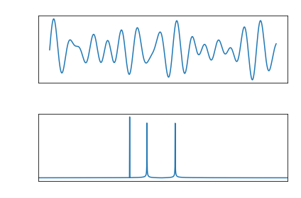
Also notice the chromagram only reveals 4 major frequencies. And because a chromagram is in the time domain, but the plot still has the same x-axis, the notes end at approximately the halfway point.
Plotting the absolute difference between MFCC features may not be visually illuminating, but potentially has uses for pattern identification. The real utility comes from comparing an audio sample to existing files. Take a look at the ascending versus ascending scales:

There is little difference in the higher coefficients, but some strong differences in the first coefficient. There are irregular differences through the rest of the plot, both in time and within coefficients. In isolation, this doesn’t reveal much. But when instead comparing two ascending scales offset by 0.1 seconds, the differences are very small. There are regular spikes in the first coefficient however, likely due to the earlier change of note in one sample.

This lack of difference is one example of how a machine learning algorithm can detect whether a audio sample fits into a group. Actually training these models will be the topic for next week.
From the blog CS@Worcester – Inquiries and Queries by James Young and used with permission of the author. All other rights reserved by the author.


