Category Archives: Independent Study

Reflection on Independent Study

With this year’s independent study presentation complete and the semester’s coming to a close, I have a project that is working. Naturally, there’s a lot more I wish I could have done. But I’ve learned a lot not only about individual technologies, but also how to plan a large project and schedule tasks.

Setting deadlines for certain portions of the project was helpful, but I did deviate from the schedule a bit in order to get more-important parts done, or prerequisite issues that were unexpectedly necessary. Some flexibility is certainly required when entering into a project without a working knowledge of the technologies at hand.

I love throwing myself into things that I know will be difficult, and that’s kind of what I was going for in this project. Turning big problems into smaller, manageable problems is one of the main reasons I enjoy software. But it’s a balancing act, because I was essentially throwing myself into 3 big problems: Learn signal processing; learn machine learning; implement a mobile application. There were a few weeks of struggling with new technologies for more hours than I had planned, and knowing that I was barely scratching the surface of only one of these big problems caused considerable stress. At times, I thought there would be no way I could get a single portion done, let alone all three.

But somehow each week I got over a new learning hump just in time to implement my goal for the week, while concurrently doing the same for my capstone sprints. Deadlines are a beautiful thing. I did a speech in my public speaking class in my first year that discussed Parkinson’s law, which says work will expand to fill the time available for its completion. This idea has followed me ever since and has proven to be true.

In preparing my presentation in the last couple of weeks, I found a couple of issues and had a couple realizations on how I could do things differently (read: better). I added some of them as I went along, and I was tempted to completely revamp the machine learning model before my presentation. Instead of the inevitable all-nighter it would have required, I managed to restrain myself and save it for the future. But this shows the importance of presenting your work as you go along, as one does in a Scrum work environment. Writing about and reflecting on issues and solutions in a simple way forced me to re-conceptualize things, both in my blog posts as I went through the semester, and in my final presentation.

While I had guidance from my advisor on how to approach and complete the project, planning and implementation was on me. There were definitely pros compared to my capstone’s team project. For example, I knew every change that was made and I had to understand all the working parts. Getting things done was mostly efficient because I only had to coordinate my own tasks. However, in my capstone I was able to bounce ideas off of team members who could provide a different perspective when we both understood the language or framework at hand. Delegating tasks also made it easier to completely understand the subtle details that allows for efficient use of a technology. Both of these experiences taught me transferable skills which I’ll be able to use in the future in solo and team projects.

From the blog CS@Worcester – Inquiries and Queries by James Young and used with permission of the author. All other rights reserved by the author.

Navigation in Android Applications

With the semester coming to a close, I have been taking all of the working pieces I have built over the past few months and began to put them together. This includes not only the Tensorflow code and the server, but also the Android application.

Having showed my current app to a few people to test the machine learning aspect, I was still presenting them with a clunky, ugly user interface with few features and poor-quality images. The user experience and interface is what I purposely saved for last.

The final app will be showcasing and describing digital signal processing techniques, as that was the focus of most of my work. As such, I had to begin setting up a way to navigate through different parts of the app and creating new “Activities” using the different “Fragments” I have created. This has been surprisingly smooth sailing so far. The tough part as been the navigation, because while it’s possible to create buttons that simply open up new pages, Android has principles that should be followed and even a Navigation component that can help define the user flow of the application.

The reason for defining navigation principles is to facilitate a consistent user experience across Android applications. For example, I have personally pressed the “Up” button on an app expecting to be brought to the previous page, but instead was brought to the Android home screen. This is a sign of poorly-maintained Activities, because previously visited pages should be on the backstack. If the Up button brings the user to the homescreen, it means the backstack was cleared at some point of previous activity.

But the user might enter a page using a deep link; going directly to a portion of the app that isn’t the normal entry point. In this case, you will still want the user to be able to return back to the standard “previous” page. To assist with this in Android, you can define a navigation graph in XML that describes how the user moves between pages. This looks very much like a user flow that should be created before implementing the app.

A top-level navigation graph
From https://developer.android.com/guide/navigation/navigation-design-graph

This also allows for nested navigation graphs, so that if one screen leads to 2 or more sections of the app, these can be defined in isolation and reused. In the image above, the “in_game” page is its own navigation graph, which the “match” screen navigates to. If the match page had a “game_options” screen, this could be another defined graph that could be linked to. Furthermore, the game options could be reached from any other pages just by linking to the defined graph. Because once in the game options, or any other portion of the app for that matter, the possible paths a user can take should not change. All in the name of consistent user experience.

With more defined in XML and handled by the Android framework, less care must be taken to monitor and control navigation through the app. While navigation components are not required in Android, it vastly simplifies the process of adhering to Android guidelines.

From the blog CS@Worcester – Inquiries and Queries by James Young and used with permission of the author. All other rights reserved by the author.

Running Server Side Code and Serving Up Some Tasty Results

Storing files on a server from a mobile app is nifty trick, but this week for my independent study I began running code on the server to extract audio features and make predictions on a spoken digit.

In its current state, my app allows a user to record an audio file. Once done, the file is uploaded to the server and will extract the audio features and submit it to the machine learning model, which currently predicts a spoken digit. The server then allows the user to look at specific information about the audio file: a graph of the certainty of which digits were spoken, the waveplot, and the MFCC features.

This basic framework allows room for growth in the future. First, I have been taking care to design the app to easily add additional features for the user’s viewing pleasure and plan on adding a spectrogram and FFT this week. Second, the machine learning model is currently trained on MFCC features only, but this can be retrained to work better using other features. And although it currently only guesses spoken digits, additional models can be trained to make a more complex system to analyze different kinds of audio data with different applications.

The biggest issue with what I’ve wanted to do in this project has been finding datasets large enough to train a model. I’d love to extend the features of the machine learning aspect of this app, but unfortunately the amount of work required is way out of scope for a single person in a single semester. Although there are many large human speech datasets, training a model in a supervised manner would require hours of manually labeling the data.

Luckily, I’ve learned enough about signal processing to make that a main aspect of the project. And as I said at the beginning of the semester, my main goal was to gain experience in the Android framework and software development in general. Having to overcome unexpected challenges and find creative ways to approach them has probably been the most important learning experience in this project.

I also continue to be reminded of the importance of knowing the shape of your data and what is actually represents before trying to work with it. MFCC features just aren’t displayed in the same way as a spectrogram or a waveplot, so each of these requires special considerations in plotting and, in the future, training machine learning models with them.

And to finish, I’d like to describe my biggest issue of the week. I had to determine how I wanted to get the data to a user after running server-side code. The naive approach would be to send all the data at once as a response, but not only would this take a long time, but the user might not want it. Instead, I send an HTTP request to get a JSON object of metadata for a given audio recording. This contains all the extracted features with a link to them for download, if desired. Then, the app itself can determine if they should be downloaded. In my case, I currently have an interface that handles the API calls, and passes back each file download link individually in a callback method when the HTTP request is successful. The app displays each link as it is received.

This week I also had to refactor an old project for an assignment and chose my first attempt at a Scrabble game in Python. The contrast between that one and this one was a reminder of the tools I’ve picked up over the past 4 years. I never would have been able to juggle this many different technologies and still understand the architecture without the help of many software engineering concepts.

From the blog CS@Worcester – Inquiries and Queries by James Young and used with permission of the author. All other rights reserved by the author.

When It’s Easier to Just Do Everything [More] Manually

Sometimes doing things the hard way is a lot easier. The more tools you use and the more complicated those tools are, the more complexity you have to deal with. So while it may be nice to call a few simple methods and have a framework do everything for you behind the scenes, you’ll have to to learn how the framework works and maybe realize down the line it can’t do everything you want it to do. There may even be incompatibilities with other parts of your program.

This week in my independent study, I tried to figure out how I could run a machine learning model on Android. I had some success, but quickly discovered some complications. Android has the option of using TensorFlow Lite, which seems great. However, I built my model using Keras, so I needed to convert the model. That was relatively straightforward, but before I started calling my model, I realized that I needed to extract audio features on Android. This required using Python code on Android, particularly Librosa and Numpy. This led me to other potential frameworks to get this to run.

This would lead to a bloated app, so I looked into Google Cloud services and thought about running server-side code there. I already set up a way to upload and download files with Google FireBase, so this seemed reasonable. But this is a paid service and would be even more work to make it functional.

I already have all the code running on my personal machine, so what if I just set up a server with a REST API to upload and download files and run the necessary Python code locally? If I could get that working, it would be trivial to call the code I’m already running.

Getting the server to upload and download files is what I did this week. I used Flask, which makes it very easy to get a basic server up and running. For the time being, data can only be transmitted via WiFi, as there will be uncompressed audio files transmitted back and forth.

While there was some additional work to figure out HTTP requests on Android, already knowing the basic building blocks gives me much more flexibility moving forward. But with great flexibility comes great responsibility, and proper error checking will be an important part of development moving forward. Security measures are also very important to consider before deploying an app to production.

The next iteration will involve running the machine learning code with a REST API call and getting back both the results of the model’s prediction and any data I will need to plot within the app.

From the blog CS@Worcester – Inquiries and Queries by James Young and used with permission of the author. All other rights reserved by the author.
Improving the Spoken Digit Speech Recognition Machine Learning Model

After getting a simple machine learning model to recognize spoken digits, I was able to begin the iterative process of improving the model. Using only MFCC’s, the model was failing more than desirable, reaching a maximum of 60% accuracy when using validation data (my own voice, which was not used in training the model).

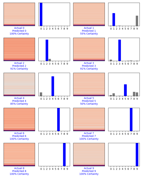
Below you will see plots of a sample of results when validating the model. For each digit, there is the extracted MFCC features, the actual spoken digit, the predicted digit by the model, and the certainty. There is also a plot of the certainty for each other digit for that recording.

This is just a sample of a larger validation set, and the actual results in this first model was only 45% accurate. But this shows that for all of these digits except 3 and 5, the model was 99% to 100% certain of the result. The differences in the MFCCs are subtle, but stark differences in color appear to be more likely to be correct, whereas 5 is clearly closer in color to 1, which it was mistake for. Additionally, every single audio clip of 3 was mistaken for a 0 using this model.

Retraining the model with different parameters may help in this case, but we can also hypothesize about the reason for these mistakes. Perhaps the MFCC is finding patterns in vowels that make “zero” and “three” look identical. If that’s the case, features that can detect consonants might help improve results. This sounds pretty obvious anyway, so it might be a good next step on the next iteration.

But first, let’s retrain the model without any changes.

Okay! This 3 was very accurately predicted. But the total accuracy of validation was only 50% (remember, this only shows a sample size of 10). Inspection of actual results now shows that 3 is sometimes mistake for a 2, and vice versa. This model is slightly better, bit still flawed. Which makes sense, because no changes have been made to the model and we just got lucky that it learned to be a bit better this time.

I’ve been training with 25 epochs, and getting 95-97% accuracy during training, and 93-97% accuracy using test data (from the same dataset as the training data, which was not used to train the model). Those results are pretty good, so maybe we can use fewer epochs and prevent some overfitting.

This certainly looks promising. With 95% accuracy during training, and 93.8% accuracy using test data, the results are still pretty good. However, the validation data with my voice is now 57.5% accurate! Only a single 3 was mistaken for a 0.

So I’m using a dataset of 4 voices to train and test, and my own voice to validate. But more data is probably better, so let’s use my voice to train the model and take a random sample to validate.

The plot is looking good! Each of these was very accurately predicted. During training and test data was 97% accurate. The validation data was 100% accurate. Of course, now that the validation data contains all voices that were trained, it’s more likely to be correct. Furthermore, the sample is small. So let’s see what happens if we use a new voice to validate. I had my roommate record himself saying each digit and used only his voice for validation data.

In general, the model is much more certain of its guesses. The final validation result was 80% accuracy, so not perfect but a major improvement. This much of an improvement was gotten just by adding more data and making small modifications to the model.

The importance of collecting data in order to improve a model is apparent. Even with 80% accuracy, there is still some predictive power. If this can be found to be useful, further data can be collected as it is used and this new data can be cleaned and used to train better models.

From the blog CS@Worcester – Inquiries and Queries by James Young and used with permission of the author. All other rights reserved by the author.

A Machine Learning Model That Recognizes Spoken Digits (Introduction)

This week, I managed to prove (to myself, at least) the power of MFCCs in speech recognition. I was quite skeptical that I could get anything to actually recognize speech, despite many sources saying how vital they are to DSP and speech recognition.

A tutorial on Tensorflow I found a couple of months ago sparked the idea: if 2-dimensional images can be represented as a 1-dimensional array and used to train the model, perhaps the same could be done with features extracted from an audio file. After all, the extracted features are nothing but an array of coefficients. So this week, armed with weeks of knowledge of basic Tensorflow and signal processing, I finally tried to get it to work. And of course, many problems arose.

After hours of struggling with mismatches in the shape of the data, waiting for the huge dataset to reload when I made a mistake, and getting no results, I finally put together the last piece of code that made it run correctly, and immediately second-guessed the accuracy of the model (“0.99 out of 100, right???”).

Of course, when training a model, a result this good could be a case of overfitting. And indeed it is, because it is only 95% accurate when using separate test data. And even this percentage isn’t the whole story. The test data comes from the same dataset, which has a lot of recordings of each digit, but using only 4 voices. It’s quite possible that there are patterns found in the voices that would not exist in other voices. This would make it great using a random sample from the original dataset, but possibly useless for someone else. There’s also the problem of noise, which MFCC is strongly affected by. So naturally, I recorded my own voice speaking digits and ran it with the model. Unfortunately, I could only manage approximately 50% accuracy, although it is consistently accurate with digits 0, 1, 2, 4 and 6. Much better than chance, at least!

This is a very simple model, which allows you to extract only MFCCs from an audio recording of a spoken digit (0 through 9) and plug it into the model to get an answer. But MFCCs may not tell the whole story, so the next step will be to use additional extracted features to get this model to perform better. There is also much more tweaking I can do with the model to see if I can obtain better results.

I’d like to step through the actual code next week and describe the steps taken to achieve this result. In the meantime, I have a lot more tweaking and refactoring to do.

I would like to mention a very important concept that I studied this week in the context of DSP: convolution. With the help of Allen Downey’s ThinkDSP and related lecture, I learned a bit more detail on filtering of signals. Convolution is essentially sweeping one signal over another to get a new signal. In DSP, this is used for things such as low-pass filters and adding echo to audio.

Think of an impulse as an instantaneous tone consisting of many (or all) frequencies. If you record this noise in a room, you will get a recording of the “impulse response”. That is, how all of the frequencies are affected by the room over time. The discrete Fourier transform of this response is essentially a filter, because it gives the amplitude of each frequency in the impulse response, including all echos and any muffling. Multiplying these amplitudes by the DFT of an entirely different audio signal will modify each frequency in the exact same way. And thus, to the human hear, this different audio signal will sound like it does in the same room. If this concept is interesting, I encourage you to watch the lecture and work through the examples in the book.

I think these topics may come in handy if I need to pre-process recordings, in the event that noise is in fact causing errors in the above model.

From the blog CS@Worcester – Inquiries and Queries by James Young and used with permission of the author. All other rights reserved by the author.

Analysis and Comparison of Ascending and Descending Scales

With added pressure in realizing the semester is half over, as well as an upcoming interview for a position dealing with DSP and machine learning, I came into this week with newfound motivation. The focus that comes with a little bit of pressure is paradoxically quite freeing.

I had some issues when attempting to compare features between audio files. In hindsight, it was an obvious mistake that I had already learned in theory. But of course, applying theoretical knowledge always reveals the points of weak understanding.

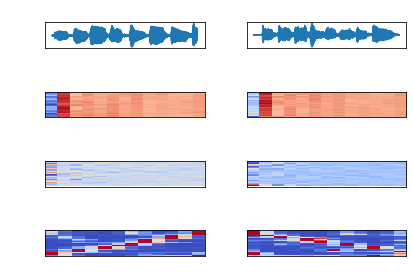
As I’ve written in the past, MFCC (mel-frequency cepstrum coefficients) are most common with speech processing. There are time slices taken from the audio file and by default Librosa calculates 13 coefficients commonly used for speech processing. The MFCC is an array of time slices, each represented by 13 coefficients. These are plotted below, with color representing magnitude (from dark blue to dark red), time slices on the y-axis, and coefficients on the x-axis. The waveform, MFCC Delta, and Chromagram are also plotted.

The chromagram is of particular interest, as it extracts the frequencies in the time domain, revealing that the scale on the left is ascending and the scale on the right is descending. You can even see where my finger slipped playing the descending scale.

Analysis of an ascending and descending scale

This shows the importance of scale invariance when comparing features, which will also come to play in machine learning. This is why frames of equal time-slices, which usually overlap, are taken from an audio sample.

Originally, I was extracting features without cutting the audio files to the same size. This resulted in a larger MFCC. Attempting to plot the difference between the features caused an error. Files with the same length, however, naturally resulted in two arrays of the same size. Because they were only slightly off, I wanted to be sure that my understanding was correct, so I made the ascending scale exactly half the size and ran the program again.

Indeed, cutting the first sample in half reveals that the resulting matrix has half as many MFCC time slices. Librosa extracts the first 13 mel-frequency coefficients, so each array will be length of 13 and each time slice will have one of these arrays. Trying to find the difference by subtracting one matrix from another results in this error message:

ValueError: operands could not be broadcast together with shapes (44,13) (87,13)
Analysis after cutting the ascending scale in half

Also notice the chromagram only reveals 4 major frequencies. And because a chromagram is in the time domain, but the plot still has the same x-axis, the notes end at approximately the halfway point.

Plotting the absolute difference between MFCC features may not be visually illuminating, but potentially has uses for pattern identification. The real utility comes from comparing an audio sample to existing files. Take a look at the ascending versus ascending scales:

The absolute difference in MFCC features between ascending and descending scales

There is little difference in the higher coefficients, but some strong differences in the first coefficient. There are irregular differences through the rest of the plot, both in time and within coefficients. In isolation, this doesn’t reveal much. But when instead comparing two ascending scales offset by 0.1 seconds, the differences are very small. There are regular spikes in the first coefficient however, likely due to the earlier change of note in one sample.

The absolute difference in MFCC features between ascending scales, offset by 0.1 seconds

This lack of difference is one example of how a machine learning algorithm can detect whether a audio sample fits into a group. Actually training these models will be the topic for next week.

From the blog CS@Worcester – Inquiries and Queries by James Young and used with permission of the author. All other rights reserved by the author.
Creating Chords from Sine Waves in Python

This week as part of my independent study I worked on feature extraction in Python. I have been using Python for Engineers as a reference, and it describes basic digital signal processing. As an exercise, I expanded on the code found in that chapter.

It’s a non-trivial task to create a sine wave in code (although compared to the most complex aspects of DSP, it’s a cakewalk). A sine wave will create the purest tone possible, as it creates a constant oscillation. This oscillation is what you perceive as a pitch. The equation for a sine wave is given as:

y(t) = A sin(2πft + φ)

where A is amplitude, f is the frequency, t is time, and φ is the phase in radians. We can ignore phase because this simply indicates where the wave starts at t=0, and this doesn’t matter to our ear. We hear the same oscillation regardless of where it starts.

Take a look a the code for creating a sine wave. Some of the details aren’t as important, but you can see the book for a description. The line that actually creates the sine wave values is:

sine_wave = [np.sin(2 * np.pi * frequency * x/sampling_rate) for x in range(num_samples)]

If you aren’t familiar with list comprehension in Python, this is just using the sine wave equation above, substituting time, t, as a specified number of samples divided by the sampling rate. The result is a list of values representing a sine wave. In reality, this is all an audio file is, with some additional encoding (and usually more interesting oscillations than a sine wave).

So what if we wanted to do this for a chord of multiple sine waves? Maybe using more list comprehension? Sure.

# Note Frequencies
a4 = 440
c5 = 523.25
e5 = 659.25
chord = [a4, c5, e5]

sine_waves = [[np.sin(2 * np.pi * freq * x/sampling_rate) for x in range(num_samples)] for freq in chord]

This is doing the same as above, only it’s doing it for each frequency in a list of frequencies. But that’s the easy part. The original code just multiplies the samples by the amplitude, then converts them to hexadecimal values and writes it to the file:

for s in sine_wave:
    wav_file.writeframes(struct.pack('h', int(s*amplitude)))

But we can’t simply do that for each sine wave in succession, or we’d get different sine waves playing one after another. That’s an arpeggio, not a chord!

So we have to get a little creative. But not too creative. If you think of each sine wave playing from a separate speaker, what you hear is the sum of the air pressure from each speaker. A single speaker is the same story: it’s just playing the sum of the three sine waves. So then, iterating through each index, we can add the amplitudes of each individual sine wave. I also had to reduce it enough to store the value as a short int, by dividing by two.

# Only write samples to the end of the shortest sine wave
shortest_sample_len = min([len(j) for j in sine_waves]) 
for i in range(shortest_sample_len): 
    current_frequencies = [wave[i] for wave in sine_waves]
    value = sum(current_frequencies) / 2
    wav_file.writeframes(struct.pack('h', int(value*amplitude)))
Output of the sums of the sin waves before multiplying by amplitude

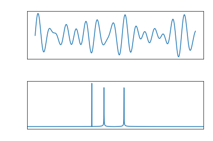
Python for Engineers goes on to describe how to use a Fast Fourier Transform to get the frequencies from the wave file with a single sine wave. But the code works just as well for the sine wave chord! This is because the FFT is an array that treats each index as a frequency, and the value at that index is the frequency’s amplitude. This means that regardless of the number of tones in a sample, the FFT can be plotted and will reveal outliers: those indices with a much higher amplitude. These are the frequencies in the audio file.

One last thing to keep in mind is that since the indices are used to represent the frequencies, they will be whole numbers. For example, c5 = 523.25hz will show up as a spike at indices 523 and 524, which 523 having the larger value of the two.

Output of finding the frequencies of the chord created above

Full code for creating a chord in Python is posted here.

From the blog CS@Worcester – Inquiries and Queries by James Young and used with permission of the author. All other rights reserved by the author.

Independent Study: The Plateau, the Snag, and the Obstacle

Researching more on audio feature extraction last week gave me a lot to think about. As it settled in, I came up with great ideas for hypothesis to test and specific applications for them. The kind of ideas that lead to turning off your cell phone, skipping lunch and dinner, and get things working.

Unfortunately, as mentioned last week, I do not have the time learn audio processing algorithms to the extent that I can implement them, so I will have to make a choice on a library that will help. A further complication was getting code to run in Android. Libraries exist to run Python code in Android, but the Python libraries I’ve found for audio analysis are lacking in features and I would need to use a combination.

The most comprehensive library I’ve found is Essentia. Of course, it’s so comprehensive I won’t be able to use the code for a professional app without a commercial license. Luckily there is a noncommercial license available that will allow me to get results for the project and determine if there are commercial applications.

Essentia is a C++ library. So the good news is I get to use JNI and the Android NDK (Native Development Kit) to run C++ code. Getting C++ code to run from an Android Activity is straightforward enough, but I do worry about potential complications in running Essentia. There are a number of dependencies that I fear might cause trouble with a feature I might want in the future. These are kept to a minimum with a special flag during compilation for Android. But alas, my paranoia strikes.

Because Essentia is open source, I am at least able to see implementations of the audio processing algorithms, and the code is well-documented with references to studies. Signal processing is a degree, not just a semester-long project. I certainly appreciate that fact more over the past couple of weeks. But this will be a great overview and using the code will still require understanding of the underlying processes.

Progress was made on converting files from audio to basic byte data. When I was considering Python libraries, I was under the assumption I could use WAV files and easily get byte data (for example, with librosa). Android’s MediaRecorder doesn’t support saving WAV files, so other formats must be used.

From the blog CS@Worcester – Inquiries and Queries by James Young and used with permission of the author. All other rights reserved by the author.

Audio Feature Extraction

This week I’ve continued working on the application part of my Android application, but I’ve also started to “dig deeper” (apprenticeship pattern blog post coming soon) and learn a bit more about audio processing.

I started with general concepts of feature extraction a couple of months ago now. Understanding how to use Python libraries to extract features is simple enough, but actually understanding how they work and why they work is another story. This week’s research has revealed an underlying elegance to the concept of signal processing and helped me reach a higher level of understanding and excitement for this project.

The single best explanation has been a video by Youtuber 3Blue1Brown on Fourier Series. I recommend all of his channel because he has an elegant way of describing and visualizing every topic he speaks about. He helped me understand the beauty of Calculus, and in my process of digging deeper I wound up watching his video on the uncertainty principle which was surprisingly relevant to signal processing. Understanding the specifics of the math behind signals and waves, and knowing the fact that mathematical equations are a language used to describe straightforward physical phenomena is key. This knowledge makes daunting concepts easier to break down. Seeing the same concepts used in different contexts also helps solidify them in your mind. And if you’re implementing this in code, it will make it much easier to remember the necessary logical steps required to extract a feature.

This entire tangent (and however useful, it was an unexpected tangent) started with trying to better understand the types of feature extraction that are used in speech recognition. By the way, you know you’re digging deeper when an article with an estimated read time of 11 minutes takes you a few hours to get through with all the additional research.

And universally, as far as I can tell, the first step in signal processing and feature extraction is the Fourier transform, which is simply turning a raw audio signal into separate sine and cosine signals. I say simply, but as the 3Blue1Brown video states, this seems a bit like figuring out which colors make up a mixed up can of paint. It turns out, however, that clever math makes it quite obvious which summation of sine and cosine signals make up a complex signal. I encourage you to watch the video to understand why.

The summation of cosine and sine waves is considered the frequency domain, while the original signal is in the time domain. From the resulting frequency domain, the individual signals can be normalized by taking the log magnitude of the signals and performing an inverse Fourier transform.

This is a new concept called a cepstrum, and it is one of many possible transformations you can make on a signal to begin to analyze the data. Its usefulness comes from the ability to see changes in individual waves. Additional operations can be performed to reveal new insights into patterns in a signal. Determining which if these works best is part of the process.

These individual transformations would be very interesting to implement in code. I may not get a chance to do so for this project, but the understanding of the underlying operations will help in using existing libraries.

From the blog CS@Worcester – Inquiries and Queries by James Young and used with permission of the author. All other rights reserved by the author.